摘要:本笔记展示了使用 decoupleR 在单细胞水平推断生物过程的方法。
# 简介
单细胞 RNA 测序 (scRNA-seq) 产生许多难以单独解释的分子读数。总结这些信息的一种方式是根据先前的知识推断出通路活性。
# 加载包
首先,我们需要加载处理 scRNA-seq 数据的 Seurat 包和使用统计方法的 decoupleR 包。
## 我们加载所需的包 | |
library(Seurat) |
Loading required package: SeuratObject

Loading required package: sp

The legacy packages maptools, rgdal, and rgeos, underpinning the sp package,
which was just loaded, will retire in October 2023.
Please refer to R-spatial evolution reports for details, especially
https://r-spatial.org/r/2023/05/15/evolution4.html.
It may be desirable to make the sf package available;
package maintainers should consider adding sf to Suggests:.
The sp package is now running under evolution status 2
     (status 2 uses the sf package in place of rgdal)


Attaching package: 'SeuratObject'

The following objects are masked from 'package:base':

    intersect, saveRDS

Loading Seurat v5 beta version
To maintain compatibility with previous workflows, new Seurat objects will use the previous object structure by default
To use new Seurat v5 assays: Please run: options(Seurat.object.assay.version = 'v5')
library(decoupleR) | |
# 仅用于数据处理和绘图 | |
library(dplyr) |
Warning: package 'dplyr' was built under R version 4.3.2


Attaching package: 'dplyr'

The following objects are masked from 'package:stats':

    filter, lag

The following objects are masked from 'package:base':

    intersect, setdiff, setequal, union
library(tibble) | |
library(tidyr) | |
library(patchwork) | |
library(ggplot2) |
Warning: package 'ggplot2' was built under R version 4.3.2
library(pheatmap) |
Warning: package 'pheatmap' was built under R version 4.3.2
# 加载数据集
这里我们使用了在 Seurat 教程 中使用的数据的下采样版本。 我们可以这样打开数据:
inputs_dir <- system.file("extdata", package = "decoupleR") | |
data <- readRDS(file.path(inputs_dir, "sc_data.rds")) |
我们可以观察到我们有不同的细胞类型:
DimPlot(data, reduction = "umap", label = TRUE, pt.size = 0.5) + NoLegend() |

# PROGENy 模型
PROGENy 是一个包含经过策划的通路和它们的目标基因及每个相互作用的权重的全面资源库。在这个示例中,我们将使用人类的权重(其他生物也可用),并且我们将使用根据 p 值排名的前 500 个响应基因。以下是每个通路的简要描述:
- 雄激素:参与男性生殖器官的生长和发展。
- EGFR:调节哺乳动物细胞的生长、存活、迁移、凋亡、增殖和分化。
- 雌激素:促进女性生殖器官的生长和发展。
- 缺氧:当氧气水平低时促进血管生成和代谢重编程。
- JAK-STAT:涉及免疫、细胞分裂、细胞死亡和肿瘤形成。
- MAPK:整合外部信号并促进细胞生长和增殖。
- NFkB:调节免疫反应、细胞因子产生和细胞存活。
- p53:调节细胞周期、凋亡、DNA 修复和肿瘤抑制。
- PI3K:促进生长和增殖。
- TGFb:参与大多数组织的发育、稳态和修复。
- TNFa:介导造血、免疫监视、肿瘤消退和防止感染。
- Trail:诱导凋亡。 - VEGF:介导血管生成、血管通透性和细胞迁移。
- WNT:在发育过程中调节器官形态生成和组织修复。
要访问它,我们可以使用 decoupleR :
net <- get_progeny(organism = 'human', top = 500) | |
net |
# A tibble: 7,000 × 4
   source   target  weight  p_value
   <chr>    <chr>    <dbl>    <dbl>
 1 Androgen TMPRSS2  11.5  2.38e-47
 2 Androgen NKX3-1   10.6  2.21e-44
 3 Androgen MBOAT2   10.5  4.63e-44
 4 Androgen KLK2     10.2  1.94e-40
 5 Androgen SARG     11.4  2.79e-40
 6 Androgen SLC38A4   7.36 1.25e-39
 7 Androgen MTMR9     6.13 2.53e-38
 8 Androgen ZBTB16   10.6  1.57e-36
 9 Androgen KCNN2     9.47 7.71e-36
10 Androgen OPRK1    -5.63 1.11e-35
# ℹ 6,990 more rows
# 使用多变量线性模型 (MLM) 进行活性推断
为了推断通路富集分数,我们将运行多变量线性模型 ( mlm ) 方法。对于我们数据集中的每个样本 ( mat ),它根据所有通路的 Pathway-Gene 相互作用权重来拟合一个线性模型,以预测观察到的基因表达。一旦拟合完成,斜率的 t 值就是分数。如果它是正的,我们解释为该通路是活跃的;如果它是负的,我们解释为该通路是不活跃的。
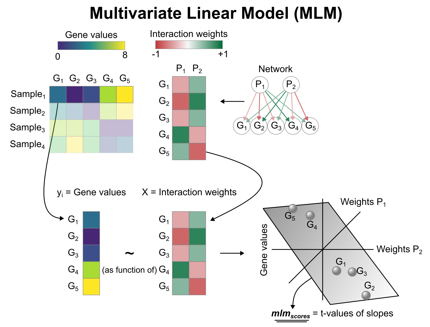
要运行 decoupleR 方法,我们需要一个输入矩阵 ( mat ),一个输入的先验知识网络 / 资源 ( net ),以及我们想要使用的 net 的列名。
# 提取标准化对数转换计数 | |
mat <- as.matrix(data@assays$RNA@data) | |
# 运行 mlm | |
acts <- run_mlm(mat=mat, net=net, .source='source', .target='target', | |
.mor='weight', minsize = 5) | |
acts |
# A tibble: 2,240 × 5
   statistic source   condition         score  p_value
   <chr>     <chr>    <chr>             <dbl>    <dbl>
 1 mlm       Androgen AAACATACAACCAC-1  0.559 0.576
 2 mlm       EGFR     AAACATACAACCAC-1  3.63  0.000290
 3 mlm       Estrogen AAACATACAACCAC-1 -0.886 0.375
 4 mlm       Hypoxia  AAACATACAACCAC-1  1.22  0.224
 5 mlm       JAK-STAT AAACATACAACCAC-1 -1.02  0.308
 6 mlm       MAPK     AAACATACAACCAC-1 -2.74  0.00619
 7 mlm       NFkB     AAACATACAACCAC-1 -0.230 0.818
 8 mlm       PI3K     AAACATACAACCAC-1 -1.09  0.276
 9 mlm       TGFb     AAACATACAACCAC-1  0.248 0.804
10 mlm       TNFa     AAACATACAACCAC-1  2.22  0.0264
# ℹ 2,230 more rows
# 可视化
从获得的结果中,我们将选择 ulm 活动并将其作为名为 pathwaysmlm 的新检测对象存储在我们的对象中:
# 提取 mlm 并将其存储在 data 中的 pathwaysmlm 中 | |
data[['pathwaysmlm']] <- acts %>% | |
pivot_wider(id_cols = 'source', names_from = 'condition', | |
values_from = 'score') %>% | |
column_to_rownames('source') %>% | |
Seurat::CreateAssayObject(.) | |
# 更改检测对象 | |
DefaultAssay(object = data) <- "pathwaysmlm" | |
# 缩放数据 | |
data <- ScaleData(data) |
Centering and scaling data matrix
data@assays$pathwaysmlm@data <- data@assays$pathwaysmlm@scale.data |
这个新的检测对象可以用来绘制活动图。在这里,我们可视化与凋亡相关的 Trail 通路,似乎在 B 和 NK 细胞中更活跃。
p1 <- DimPlot(data, reduction = "umap", label = TRUE, pt.size = 0.5) + | |
NoLegend() + ggtitle('celltype') | |
p2 <- (FeaturePlot(data, features = c("Trail")) & | |
scale_colour_gradient2(low = 'blue', mid = 'white', high = 'red')) + | |
ggtitle('Trail activity') |
Scale for colour is already present.
Adding another scale for colour, which will replace the existing scale.
p1 | p2 |

# 探索
我们还可以看到不同组在各通路上的平均活性:
# 从对象中提取活动数据作为长格式的数据框 | |
df <- t(as.matrix(data@assays$pathwaysmlm@data)) %>% | |
as.data.frame() %>% | |
mutate(cluster = Idents(data)) %>% | |
pivot_longer(cols = -cluster, names_to = "source", values_to = "score") %>% | |
group_by(cluster, source) %>% | |
summarise(mean = mean(score)) |
`summarise()` has grouped output by 'cluster'. You can override using the
`.groups` argument.
# 转换为宽格式矩阵 | |
top_acts_mat <- df %>% | |
pivot_wider(id_cols = 'cluster', names_from = 'source', | |
values_from = 'mean') %>% | |
column_to_rownames('cluster') %>% | |
as.matrix() | |
# 选择色彩调色板 | |
palette_length = 100 | |
my_color = colorRampPalette(c("Darkblue", "white","red"))(palette_length) | |
my_breaks <- c(seq(-2, 0, length.out=ceiling(palette_length/2) + 1), | |
seq(0.05, 2, length.out=floor(palette_length/2))) | |
# 绘图 | |
pheatmap(top_acts_mat, border_color = NA, color=my_color, breaks = my_breaks) |

在这个具体示例中,我们可以观察到 Trail 在 B 和 NK 细胞中更活跃。
# 工作环境
sessionInfo() |
R version 4.3.1 (2023-06-16 ucrt)
Platform: x86_64-w64-mingw32/x64 (64-bit)
Running under: Windows 11 x64 (build 22621)

Matrix products: default


locale:
[1] LC_COLLATE=Chinese (Simplified)_China.utf8
[2] LC_CTYPE=Chinese (Simplified)_China.utf8
[3] LC_MONETARY=Chinese (Simplified)_China.utf8
[4] LC_NUMERIC=C
[5] LC_TIME=Chinese (Simplified)_China.utf8

time zone: Asia/Hong_Kong
tzcode source: internal

attached base packages:
[1] stats     graphics  grDevices utils     datasets  methods   base

other attached packages:
 [1] pheatmap_1.0.12         ggplot2_3.4.4           patchwork_1.1.2
 [4] tidyr_1.3.0             tibble_3.2.1            dplyr_1.1.3
 [7] decoupleR_2.9.1         Seurat_4.9.9.9058       SeuratObject_4.9.9.9091
[10] sp_2.0-0

loaded via a namespace (and not attached):
  [1] RColorBrewer_1.1-3     rstudioapi_0.15.0      jsonlite_1.8.7
  [4] magrittr_2.0.3         spatstat.utils_3.0-3   farver_2.1.1
  [7] rmarkdown_2.23         vctrs_0.6.3            ROCR_1.0-11
 [10] spatstat.explore_3.2-1 htmltools_0.5.5        progress_1.2.2
 [13] curl_5.0.1             cellranger_1.1.0       sctransform_0.3.5
 [16] parallelly_1.36.0      KernSmooth_2.23-21     htmlwidgets_1.6.2
 [19] ica_1.0-3              plyr_1.8.8             plotly_4.10.2
 [22] zoo_1.8-12             igraph_1.5.0           mime_0.12
 [25] lifecycle_1.0.3        pkgconfig_2.0.3        Matrix_1.6-1.1
 [28] R6_2.5.1               fastmap_1.1.1          fitdistrplus_1.1-11
 [31] future_1.33.0          shiny_1.7.4.1          selectr_0.4-2
 [34] digest_0.6.33          colorspace_2.1-0       tensor_1.5
 [37] RSpectra_0.16-1        irlba_2.3.5.1          labeling_0.4.2
 [40] progressr_0.13.0       fansi_1.0.4            spatstat.sparse_3.0-2
 [43] httr_1.4.6             polyclip_1.10-4        abind_1.4-5
 [46] compiler_4.3.1         bit64_4.0.5            withr_2.5.0
 [49] backports_1.4.1        logger_0.2.2           fastDummies_1.7.3
 [52] OmnipathR_3.8.2        MASS_7.3-60            rappdirs_0.3.3
 [55] tools_4.3.1            lmtest_0.9-40          httpuv_1.6.11
 [58] future.apply_1.11.0    goftest_1.2-3          glue_1.6.2
 [61] nlme_3.1-162           promises_1.2.0.1       grid_4.3.1
 [64] checkmate_2.3.1        Rtsne_0.16             cluster_2.1.4
 [67] reshape2_1.4.4         generics_0.1.3         gtable_0.3.3
 [70] spatstat.data_3.0-1    tzdb_0.4.0             hms_1.1.3
 [73] data.table_1.14.8      xml2_1.3.5             utf8_1.2.3
 [76] spatstat.geom_3.2-4    RcppAnnoy_0.0.21       ggrepel_0.9.3
 [79] RANN_2.6.1             pillar_1.9.0           stringr_1.5.0
 [82] vroom_1.6.3            spam_2.9-1             RcppHNSW_0.4.1
 [85] later_1.3.1            splines_4.3.1          lattice_0.21-8
 [88] bit_4.0.5              survival_3.5-7         deldir_1.0-9
 [91] tidyselect_1.2.0       miniUI_0.1.1.1         pbapply_1.7-2
 [94] knitr_1.45             gridExtra_2.3          scattermore_1.2
 [97] xfun_0.39              matrixStats_1.0.0      stringi_1.7.12
[100] lazyeval_0.2.2         yaml_2.3.7             evaluate_0.21
[103] codetools_0.2-19       cli_3.6.1              uwot_0.1.16
[106] xtable_1.8-4           reticulate_1.30        munsell_0.5.0
[109] readxl_1.4.3           Rcpp_1.0.11            globals_0.16.2
[112] spatstat.random_3.1-5  png_0.1-8              parallel_4.3.1
[115] ellipsis_0.3.2         readr_2.1.4            prettyunits_1.1.1
[118] dotCall64_1.0-2        listenv_0.9.0          viridisLite_0.4.2
[121] scales_1.2.1           ggridges_0.5.4         leiden_0.4.3
[124] purrr_1.0.2            crayon_1.5.2           rlang_1.1.1
[127] rvest_1.0.3            cowplot_1.1.1